When performing research it is essential that you are able to make sense of your data. This allows you to inform other researchers in your field and others what you have found. It also can be used to build evidence for a theory. Therefore an understanding of what test to use and when is necessary. There are some good practices to do if you are not familiar with performing statistical analysis. The first is to determine your variables.
Overview of basic statistics:
- 1. Dependent variable (DV)-This is the one that you are measuring. From the example of the student's score.
- 2. Independent variable (IV)-This is the one that you are manipulating with the different conditions. From the example either PowerPoint or overhead projector presentation (Aron, Aron, & Coups, 2005).
Levels of Measurement:
Once this has been done you will want to determine the level of measurement that both variables are. This will assist you later determine what test to use in your analysis. There are four levels of measurement (Aron, Aron, & Coups, 2005):- 1. Interval-There is no true zero, there are equal intervals throughout the scale, and negative scores are possible (i.e. 80.5 degrees Fahrenheit).
- 2. Ratio-There are equal intervals throughout the scale, and has a true zero so negative scores are not possible (i.e. 1 marble).
- 3. Nominal-Categories (i.e. Male/Female).
- 4. Ordinal-Ranking (i.e. 1st, 2nd, 3rd, and 4th).
With this information you can refer to the following chart to determine what statistical test to use (see Figure 1).
Figure 1. Chart of tests by design, number of conditions, and level of measurement
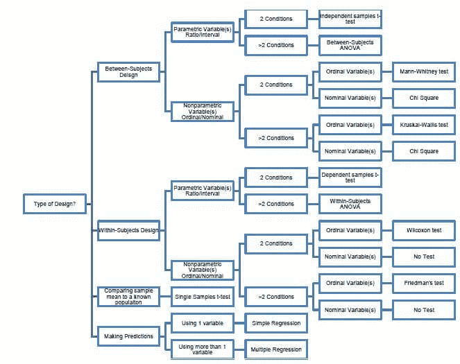
Statistical tests can be broken into two groups, parametric and nonparametric and are determined by the level of measurement, number of dependent and independent variables, covariates, comparing to an already known population, and type of design. Parametric tests are used to analyze interval and ratio data, and nonparametric tests analyze ordinal and nominal data. There are different tests to use in each group. We will start with the parametric tests first.
Parametric Tests: (Interval/Ratio data)
These tests assume that the data is normally distributed (bell curve) and are very strong when compared to nonparametric tests (Heiman, 2001).1. Within-Subject Design
- A. Paired-Samples t-Test (AKA: Dependent samples t-test): Compares means of two groups who received all conditions (Aron, Aron, & Coup, 2005). An example is having participants run a mile one day with no sleep and then with a full night's sleep, and seeing which group was the fastest.
- B. Within-subjects ANOVA (AKA: Repeated-Measures ANOVA): Compares means of more than two groups who received all conditions, and decreases the rate of Type I errors (described later in this section)(Aron, Aron, & Coup, 2005 & Cronk, 2011). An example is having participants run a mile one day with no sleep, a full night's sleep, and with caffeine prior to run.
- A. Independent samples t-test: Compares means of two groups (Aron, Aron, & Coup, 2005). An example is determining if a PowerPoint presentation impacted grades compared to a control group, that received a general lecture.
- B. Between-subjects ANOVA (AKA: One-Way ANOVA): Compares means of more than two groups, and participants only receive one of the conditions (Cronk, 2011). An example is determining if PowerPoint or an overhead projector impacted grades and if so which one.
- C. Pearson Correlation: Determines if there is a relationship between two variables (NOT CAUSATION). It also determines the strength of the relationship, if one exists (Aron, Aron, & Coup, 2005).
- D. Factorial ANOVA: Compares means of more than two groups, each with multiple levels in the independent variable (Cronk, 2011). An example is determining if patients' health improved using one of four different antibiotics either with intravenous fluids or not. In this case it would be called a 4 x 2 factorial ANOVA, because there are two independent variable (antibiotics and intravenous fluids). The first independent variable has four levels (antibiotics) and the second independent variable has two levels (intravenous fluids).
- 3. Mix Design
- A. Mix-Design ANOVA: Compares means of more than two groups, with multiple independent variables (Cronk, 2011). One independent variable must be within-subjects (repeated measures) and one must be between-subjects.
- 4. Comparing Means
- A. Single-Sample t-Test (AKA: z-Test): Compares the mean of one sample against the mean of an already known population (Aron, Aron, & Coup, 2005). An example would be comparing the ACT scores of students in one state against that of the entire country.
- 5. Covariates
- Covariates are variables which are in some way related to the dependent variable, however are not considered to be independent variables (Cronk, 2011). An example is the effect of gender on reaction time while considering age. Here gender would be the covariate as gender is related to reaction time scores.
- A. ANCOVA: Compares the means of more than two groups, and allows researchers the ability to remove a covariate (Cronk, 2011). As stated before an example is the effect of gender and age on reaction time. The researcher could remove gender as it is known it is related to reaction time.
- 6. More than One Dependent Variable
- In some cases, researchers may have more than one dependent variable. An example is determining the effect of treatment type (chemotherapy, radiation therapy, or combination on both) on tumor markers and tumor size.
- A. MANOVA: Compares the means of more than two groups when there is more than one dependent variable, and decreases Type I error (Cronk, 2011). As stated before an example is the effect of treatment type (chemotherapy, radiation therapy, or combination on both) on tumor markers and tumor size.
- A. Wilcoxon: This is the nonparametric version of the dependent samples t-test as it compares the difference of ranks for groups of two with ONLY ordinal data (Cronk, 2011). An example is determining participants' ranking for visual preference between two iPad game apps.
- B. Friedman: This is the nonparametric version of the within-subjects ANOVA as it compares ranks for groups of more than two with ONLY ordinal data (Cronk, 2011). An example is determining the rank of three different websites based on user friendliness.
- A. Chi Square: Compares ranks for both two group and more than two group designs with ONLY nominal data (Aron, Aron, & Coup, 2005).
- 1. Chi square Goodness of Fit-Compares the proportion of the sample to an already existing value. An example would be comparing literacy rates in central Missouri against those of the entire state.
- 2. Chi Square Test of Independence-Compares the proportions of two variables to see if they are related or not. An example would be are there similar numbers of baseball and softball athletes enrolled in this semester's general psychology course.
- B. Kruskall-Wallis: This is the nonparametric version of the between-subjects ANOVA as it sees if multiple samples are from the same population (Cronk, 2011). An example is determining how participants rate a physician based on whether he/she used a computer, book, or no assistance in diagnosing them.
- C. Mann-Whitney: This is the nonparametric version of the independent samples t-test as it compares ranks for groups of more than two with ONLY ordinal data (Cronk, 2011). An example would be determining if eating Snickers candy bars affects students' grades in math courses.
- D. Correlations:
- 1. Spearman's Rho: Like the Pearson correlation, this test too determines the strength of the relationship between two variables based on their ranks. An example would be to determine the relationship between physics and English course grades.
- 1. Simple Linear Regression: This is when one known variable is used to predict the value of another variable (Cronk, 2011). An example would be using a student's GRE scores to predict their graduate school GPA.
- 2. Multiple Linear Regression: This is when more than one variable is used to predict the value of another variable (Aron, Aron, & Coup, 2005). An example would be temperature, wind speed, and humidity to predict the amount of precipitation that will fall.
- A. Null hypothesis: This states that there is NO statistical significance between the groups.
- B. Alternative hypothesis: This states that there IS a statistical significance between the groups.
- 1. Type I error: The alternative hypothesis is accepted when the null hypothesis is actually true.
- 2. Type II error: The null is accepted when in fact the alternative hypothesis is true (see Table 3).
2. Between-Subject Design
The correlation coefficient (r) ranges from -1.0 to 1.0. The closer to -1.0 or 1.0, the stronger the relationship. When r is negative, that means there is a negative relationship (one variable goes up or down the other does the opposite). When r is positive, that means there is a positive relationship (one variable goes up or down so does the other). See the example below examining the correlation between texts sent per week and grades. Another way to determine the relationship and strength is to look at the graph. The closer the data points are to the line, the stronger the relationship (see Figure 2) (Heiman, 2001).
Caution: A strong correlation does not mean that a condition caused the outcome. It only means that the two variables are related in some way.
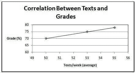
Figure 2. Graph of texts vs. grade correlation
Nonparametric Tests: (Ordinal/Nominal data)
These tests do not assume anything about the shape of the data. These tests are not as strong as the parametric ones (Heiman, 2001).1. Within-Subject Design
2. Between-Subject Design
Prediction:
In some cases, a researcher may want to use one or more variables to predict another variable. In this case, the researcher would use a regression.
Hypothesis Types:
In research there are two main hypotheses (Aron, Aron, & Coups, 2005):
Error Types:
No matter how well a study is designed there is always the probability that chance is what caused the results, not the different treatments. When a researcher accepts results that are not accurate it is called an error . There are two main types of error (Aron, Aron, & Coups, 2005):
Table 3. Accept/reject the null when it was either true/false
| True | False | |
|---|---|---|
| Accept Null | Good decision | Type I |
| Reject Null | Type II | Good decision |
REFERENCES
Aron, A., Aron, E., & Coups, E. (2005). Statistics for psychology (4th ed.). Pearson, pgs 4, 176-177, 223, 236, 270, 506, 539, 634.
Cronk, B. (2011). How to use SPSS (7th ed.). Pyrczak, pgs 50, 59, 65, 69, 74, 77, 81, 85, 87, 101, 105, 108, 113, 131.
Heiman, G. (2001). Research Methods in Psychology (3rd ed.). Cengage Learning, pgs 206-207 & 271-272.
